
The geography of work, wages and gender
Associate Professor of Economics and Finance, University of Indianapolis
The question seems simple enough: Are there discernable wage differences among individuals experiencing spells of unemployment upon reemployment and if so, does mobility make a difference and if it does, what types of differences result due to gender? This article is a summary of research conducted to answer that question.
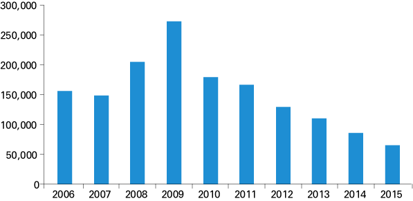
For our study, we used a longitudinal data set of de-identified unemployment claimant data that comprises a ten-year period of individuals receiving unemployment benefits and followed their reemployment using quarterly wage records.1 This data set allowed us to assess individual periods of unemployment as an exogenous shock on wages and thereby determine the underlying influences in the labor market. The number of records, or observations, in the data set are enumerated in Figure 1.
Figure 1: Number of observations used in study
Source: Author's calculations
Research abounds showing that spells of unemployment can negatively affect income and wages. For most workers, getting back to work quickly after a layoff, or finding a new job after losing one, is imperative. But for some unemployed workers, their skills may not match the needs of local businesses. As a result, some people will need to go beyond their local area for work and that requires a longer commute–which, in turn, requires additional time and transportation. For workers who can’t embark on a longer commute, the stretch of time from unemployment to reemployment may take longer. This can eventually result in taking a job with the advantage of being closer to home, but the disadvantage of lower wages.
The literature on gender-wage disparity is robust. While much of the existing literature focuses on symptom assessment, there has been less focus on source identification. One area of source research on gender-wage disparity examines gender and job transfer [33-35].
Geographic mobility and spatial wage studies examine both physical relocation and allotments for commuting time. Mills [36] and Muth [37] address the issue of firm migration from city centers and resulting wage impacts. Rees and Schultz [38] investigate the wage differences of city-center employment versus their suburban counterpart.
Women often carry increased family responsibilities that affect their ability to relocate or commute extensively for employment [39-42]. The concern is that the limitation of geographic mobility becomes a gender trap for lower wages. Prior research supporting this thesis focuses on city-center versus suburban employment [43,44].
Our study adds to existing research by applying a novel approach to wage analysis. It uses administrative wage data and unemployment shocks to assess the link between geographic mobility and wages. The study supports prior results when assessing short-distance mobility, described as micro-mobility. In this case, micro-mobility is the movement between Indiana counties measured in kilometers. The study also broadens the thesis by expanding the argument beyond the “city center versus suburban” framework that currently dominates the literature. The gender divergence of geographic mobility partially explains the gender disparity in wages. Numerous factors, including family considerations, limit mobility and detrimentally influence wages. As females often carry a disproportionate weight of those family considerations, they also carry its wage influence.
The data set used ascertains the individual’s wages before and after each episode of unemployment and includes observations from the first quarter of 2006 through the Great Recession and subsequently, the fourth quarter of 2015. Portions of the data set came from individuals when applying for unemployment benefits. Each incidence of unemployment is a unique claims episode, and individuals may appear multiple times during the collection period. In an effort to protect record unanimity, information about repeat episodes of unemployment is not available.2
This research examined the wage impact of workforce reintegration using a data set aggregated from administrative wage and unemployment data. Those data did not include the self-employed, Indiana residents working in another state or individuals coming into Indiana for employment. The data set was also constrained around the ages of 18 to 80. All calculations are those of the author.
Findings
The results indicate a positive relationship between post-unemployment wages and mobility. Micro-level mobility, or movement over short distances within Indiana, positively affects wages. In fact, an increase of one kilometer in mobility is associated with a gain of $0.34 in quarterly wages.
High wages prior to unemployment and a long duration of unemployment increase the potential for lower wages in a new job. The higher the wages were prior to the period of unemployment, the more likely post-unemployment wages will be reduced. Likewise, the longer someone is unemployed, the more detrimental that unemployment is on their future wages.
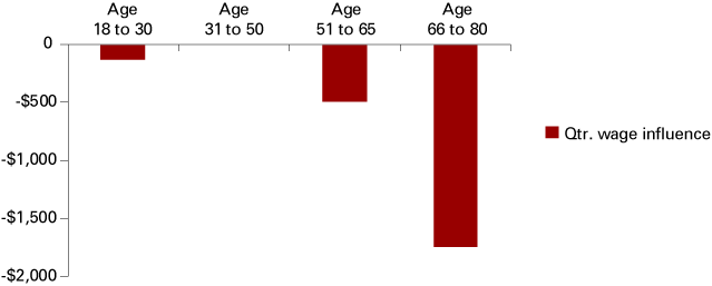
The gender variable also yields significant results for post-unemployment wages. The results indicate that males reemploy with less of a wage discount. In fact, the difference between male and female quarterly wages is $793.10. The impact of the wage differential based on race is comparatively modest. Age, however, does play a factor. Wages are discounted progressively more for those in the older age brackets. Figure 2 illustrates the age bias on unemployment discounts.
Figure 2: Age bracket influence on unemployment discount
Source: Author's calculations
Finding employment with the same employer or in the same industry is beneficial in maintaining a comparable wage post-unemployment. By returning to the same place of employment and maintaining the same line of work, an individual can leverage their skills and knowledge to achieve a better wage when reattaching to the workforce.
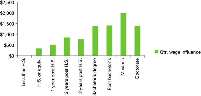
Education is also a large influence on the ability of an individual to successfully navigate unemployment and achieve higher wages after workforce reattachment. Increasing levels of education produce higher wages in the reemployment market, as seen in Figure 3.
Figure 3: Education influence on unemployment discount
Source: Author's calculations
Finally, the occupation held before unemployment is an important determinant on subsequent post-unemployment wages. Training and experience are influential factors on the unemployment experience.
Implications
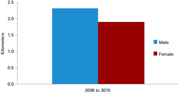
The results indicate that geographic micro-mobility over short distances (kilometers) is a source of wage disparity in the reemployment market. Mobility rates vary by demographic category, which can be a source of consistent wage inequality. The study examines the differing rates of mobility by gender. The rates of micro-mobility between genders in the data set differ by an average of approximately 22% (Figure 4). While the magnitude of the mobility is incrementally small, the aggregated effect compounded over a lifetime can partially explain the consistent wage disparity found in prior research.
Figure 4: Micro-mobility: Additional kilometers to new job
Source: Author's calculations
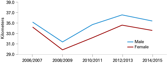
The study further assessed two-year increments of data. This is done both as a robustness check and to determine if the results vary over time. Within the two-year segments, males typically express greater rates of geographic micro-mobility before unemployment. Figure 5 indicates the distance (in kilometers) to the place of employment prior to the episode of unemployment. The economic crisis of 2008-2009 affected workers increasingly close to their residence. The gap between micro-mobility rates by gender remains relatively constant.
Figure 5: Distance from residence to old job (in kilometers)
Source: Author's calculations
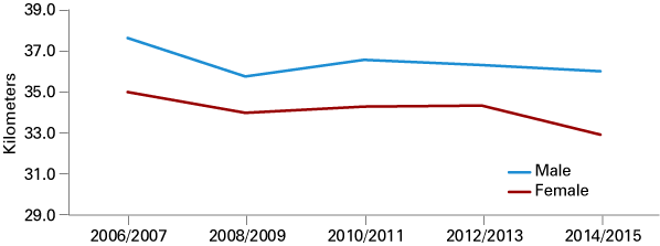
Figure 6 indicates geographic micro-mobility rates of the unemployed after reattachment to the labor market. The figure indicates the distance (in kilometers) to the place of employment post-unemployment. Again, a persistent gender gap in mobility rates exists. Upon close examination, there is a slight narrowing of the mobility gender difference during the middle three periods compared to the first and last periods. Behavior becomes increasingly similar during economic distress. Before and after economic distress, the gender gap widens.
Figure 6: Distance from residence to new job (in kilometers)
Source: Author's calculations
Geographic micro-mobility is an important factor in determining post-unemployment wages. Limiting the job search to a specific location or approximate vicinity is detrimental to post-unemployment wages. Mobility may partially explain lingering wage gaps for certain segments of society, such as women. Household commitments and other considerations may limit female geographic mobility, which hinders wage attainment and allows for persistent wage gaps. The effect is evidenced in the reemployment market, but may extend into the overall labor market. An extension of this analysis could assess the effects of geographic micro-mobility on other demographic factors.
More on methodology
A wage variable measured the difference between an individual’s wages entering the claims system against the wages once reintegrated into the labor market. The wage difference is as follows:
Wage difference = (Avg. wages post-UI claim) – (Avg. wages pre-UI claim)
A positive wage difference reflects higher wages after the episode of unemployment, while a negative wage difference reflects decreased wages after unemployment. The wage difference is the dependent variable in the regression analysis.
Independent variables assess influence on the wage discount. The study focuses on county-to-county mobility within Indiana, or micro-mobility.3 To assess the impact, a variable measures the movement of individuals during episodes of unemployment. The county of residence of the unemployed individual prior to the episode is self-reported when applicants apply for unemployment benefits. Indiana wage records contain the location of the employer both pre-and post-unemployment episode.
A constructed 92 x 92 diagonal matrix compares geographic midpoint distances between all Indiana counties. For each unemployment episode, the distance (in kilometers) from the individual’s residence to the employer prior to the unemployment episode is determined from the matrix. If it is the same county, the distance is zero. The distance from residence to the employer post-unemployment episode is also determined using the same methodology. The distance between the pre- and post-unemployment episode serves as a proxy for the increased willingness of an individual to commute or move for employment. The distance difference equation is as follows:
Kilometers to new job = (Kilometers post-UI episode) – (Kilometers pre-UI episode)
A positive difference reflects an individual willing to travel further for a new position (increased mobility). A negative difference reflects a new position closer to the individual’s residence. Zero indicates no difference in distances.4
The earning power of an individual prior to an episode of unemployment is a likely influence on the wage difference, so a “wage before unemployment” variable is added.5
The total time collecting UI benefits is the total number of weeks UI benefits were received. The resulting variable, “total weeks of unemployment claimed,” includes all benefits, including state and federal.6
Explanatory variables include claimant characteristics such as gender, age and race/ethnicity. The variables are self-reported when applicants apply for unemployment benefits. A binary gender variable (Gender Male) is included and is affirmative for male. A binary variable (White) results from individuals self-reporting as white or Caucasian. The observations segregate into the following binary age categories:
- Ages 18 to 30
- Ages 31 to 50
- Ages 51 to 65
- Ages 66 to 80
When individuals experience unemployment, they often attempt to reattach in positions similar to previous employment to maximize knowledge and experience. In some instances, such as temporary layoffs, an unemployed person may reattach with their previous employer. A binary variable (Same Employer) is affirmative if the individual reattaches with the same employer they had prior to unemployment. If the person cannot find employment at the same firm, they may attempt to leverage their knowledge in the same field. A binary variable (Same Industry NAICS) is included, in case the individual reattaches with a new employer in the same industry as prior employment, as denoted by a common two-digit NAICS code. The Indiana yearly gross domestic product (GDP) variable controls for the economic environment during unemployment. Yearly binary variables account for yearly variation.
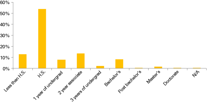
The highest level of educational attainment achieved by the unemployed is also included as binary variables. Education is self-reported when applicants apply for unemployment benefits. Figure 7 shows the education level of applicants. The data skew toward lower educational attainment levels, as the probability of unemployment increases with decreased education.
Figure 7: Educational attainment achieved by individuals in the data set
Source: Author's calculations
Occupational variables are also included. The Standardized Occupational Code (SOC) is self-reported when applicants apply for unemployment benefits. It represents the position of the applicant at separation. Unfortunately, the SOC for new positions are not available.
Regional differences are likely to affect the unemployment experience. The Indiana Department of Workforce Development (IDWD) divides the state into 12 Economic Growth Regions (EGRs) by counties clustered by economic commonality. Binary variables are created (Home EGR) to indicate the individual’s home location.
The study's main finding about post-unemployment wages is this: During the period of 2006 to 2015, an individual going through a period of unemployment in Indiana received on average $431.06 less per quarter (or $1,724.24 annually) in their new position as compared to their prior employment.
Notes
- A random identifier is applied and the researcher never has access to identified data, ensuring record anonymity. The results are provided in aggregate.
- The data was requested, but was prohibited due to privacy concerns. The data would be helpful as many of the unemployment claimants may appear multiple times in the data set.
- Location by zip or other method of granularity is not permitted due to privacy concerns.
- Data by zip code is preferred, but not allowed due to anonymity concerns. It is acknowledged that some people may move resulting from job displacement. Therefore, it is not assumed that this variable only shows an increase in commuting time. It is also acknowledged that there are discrepancies in recorded counties for residence of both the individuals and companies (particularly if the company operates physical locations in multiple counties).
- This represents the average of the second and third quarters preceding unemployment. As the quarter directly preceding unemployment is likely a partial quarter, it is discarded.
- Some federal benefits programs, particularly those covered by the Trade Adjustment Assistance Program, can extend for a very long period during re-training. However, these types of extended programs are infrequent.
Acknowledgements
Contributors to the whitepaper (and by extension, this article) include professors from the University of Indianapolis Allison Snyder (School of Business) and Amanda Miller (Department of Sociology), Timothy Slaper and Vicki Seegert with the Indiana Business Research Center and Charles Baer and Lori Wasson with the Indiana Department of Workforce Development.
References used in the full whitepaper
[1] Deavers, K. “Rural America: Lagging Growth and High Poverty…Do We Care?” Choices 4, no. 2 (1989): 4-7.
[2] Duncan, C.; Tickamyer, A. “Poverty Research and the Policy for Rural America.” American Sociological Review 19, no. 3 (1988): 243-259.
[3] Levy, F. Dollars and Dreams: The Changing American Income Distribution. New York: Russell Sage, 1987.
[4] Tickamyer, A.; Duncan, C. “Work and Poverty in Rural America.” In Rural Policy for the 1990’s. Edited by J. Christenson, D. Flora. Boulder/London: Westview, 1990.
[5] Williams, T.; Kornblum, W. Growing Up Poor. Lexington, Mass: Heath, 1985.
[6] Kuznets, S. “Economic Growth and Income Inequality.” American Economic Review 45 (1955): 1-28.
[7] Williamson, J. “Regional inequality and the Process of National Development: A Description of Patterns.” Economic Development and Cultural Change 13 (1965): 3-45.
[8] Barrios, S.; Strobl, E. The Dynamics of Regional Inequalities. Economic Papers of the European Commission, p. 229. Brussels: 2005.
[9] Ezcurra, R.; Pascual, P. “Regional Polarisation and National Development in the European Union.” Urban Studies 44, no. 1 (2007): 99-122.
[10] Myrdal, G. Economic Theory and Underdeveloped Regions. Hutchinson, 1957.
[11] Fleming, J. “External Economics and the Doctrine of Balanced Growth.” Economic Journal 65 (1955): 241-256.
[12] Hirschman, A. The Strategy of Economic Development. New Haven, Conn.: Yale University Press, 1958.
[13] Segal, D. “Are There Returns of Scale in City Size?” Review of Economics and Statistics 89 (1976): 393-413.
[14] Henderson, A. Urban Development. Oxford University Press, 1958.
[15] Card, D. “The Casual Effect of Education on Earnings.” Chapter 30 in O. Ashenfelter and D. Card (Eds.) Handbook of Labor Economics, Vol 3. Amsterdam: Elsevier, 1999.
[16] Tilak, JBG. Education and Its Relation to Economic Growth, Poverty, and Income Distribution: Past Evidence and Future Analysis. Washington D.C.: World Bank, 1989.
[17] Goldin, C.; Margo, RA. “The Great Compression: The Wage Structure in the United States at Mid-Century.” Quarterly Journal of Economics 107 (February 1992): 1-34.
[18] Teulings, CN. “The Wage Distribution Model of the Assignment of Skills to Jobs.” Journal of Political Economy 103, no. 2 (1995): 280-315.
[19] Teulings, CN. “Comparative Advantage, Relative Wages, and the Accumulation of Human Capital.” Journal of Political Economy 113, no. 2 (2005): 425-461.
[20] Acemoglu, D. “Technical Change, Inequality, and the Labor Market.” Journal of Economic Literature (March 2002): 7-72.
[21] Blackburn, ML. “What Can Explain the Increase in Earnings Inequality Among Males?” Industrial Relations 29 (1990): 441-456.
[22] Bound, J.; Johnson, G. “Changes in the Structure of Wages in the 1980’s: An Evaluation of Alternative Explanations.” American Economic Review 82 (June 1992): 371-392.
[23] Karoly, LA. “Changes in the Distribution of Individual Earnings in the United States: 1967-1986.” Review of Economics and Statistics 74 (February 1992): 107-115.
[24] Katz, LF; Murphy, KM. “Changes in Relative Wages, 1963-1987: Supply and Demand Factors.” Quarterly Journal of Economics 107 (1992): 35-78.
[25] Kosters, M. Workers and Their Wages: Changing Pattern in the United States. Washington D.C.: American Enterprise Institute, 1991.
[26] Mehta, SR. “Quality of Education, Productivity Changes, and Income Distribution.” Journal of Labor Economics 18, no. 2 (April 2000): 252-281.
[27] Thurow, L. “A Surge in Inequality.” Scientific American 256, no. 5 (May 1987): 26-33.
[28] Revenga, AL. “Exporting Jobs?” Quarterly Journal of Economics 107 (February 1992): 255-284.
[29] Dickens, WT; Lang, K. “A Test of Dual Labor Market Theory.” American Economic Review 75 (September 1985): 792-805.
[30] Dickens, WT; Lang, K. “Where Have all the Good Jobs Gone? Deindustrialization and the Labor Market Segmentation.” In Unemployment and the Structure of Labor Markets”. Edited by K. Lang and J. Leonard. New York: Blackwell, 1987.
[31] Singelmann, J. From Agriculture to Services: The Transformation of Industrial Employment. Beverly Hills, CA.: Sage, 1987.
[32] Tienda, M. Industrial Restructuring in Metropolitan and Nonmetropolitan Labor Markets: Implications for Equity and Efficiency. See Killian et. al.; 1986. p. 33-70.
[33] Loprest, PJ. “Gender Differences in Wage Growth and Job Mobility.” The American Economic Review 82, no. 2 (May 1992): 526-532.
[34] Keith, K.; McWilliams, A. “The Returns to Mobility and Job Search by Gender.” ILR Review 52, no. 3 (April 1999): 460-477.
[35] Fuller, S. “Job Mobility and Wage Trajectories for Men and Women in the United States.” American Sociological Review 73, no. 1 (February 2008): 158-183.
[36] Mills, ES. Studies in the structure of the urban economy. Baltimore: John Hopkins University Press, 1972.
[37] Muth, RF. Cities and housing: The spatial patterns of urban residential land use. Chicago: University of Chicago Press, 1969.
[38] Rees, A.; Schultz, GP. Workers and wages in an urban labor market. Chicago: University of Chicago Press, 1970.
[39] Carlson, VL. The availability of women workers: The effects on company location in the suburbs. New York: Garland, 1997.
[40] Hanson, S.; Pratt, G. “Spatial dimensions of the gender division of labor in a local labor market.” Urban Geography 9 (1988): 367-78.
[41] Hanson, S.; Pratt, G. “Job search and the occupational segregation of women.” Annals of the Association of American Geographers 81 (1991): 229-53.
[42] Nelson K. “Labor demand, labor supply and the suburbanization of low-wage office work.” In Production, work, territory: The geographical anatomy of industrial capitalism. Eds. A. Scott and M. Storper, Boston: Allen Unwin, 1986. p. 149-69.
[43] Madden JF. “Why women work closer to home.” Urban Studies 18 (1991): 181-94.
[44] Ihlanfeldt KR. “Intraurban wage gradients: Evidence by race, gender, occupational class, and sector.” Journal of Urban Economics 32 (1992): 70-91.


