
The Importance of Education for the Unemployed
Based on a working paper
Professor of Economics and Finance, University of Indianapolis
Co-Director, The Center of Excellence in Workforce Education Research
What is the short-term influence of education in the re-employment market? Does it help people regain employment after receiving unemployment insurance benefits?
To answer these questions, this analysis uses unique employment and unemployment claims data and a simple model. The model attempts to determine which factors impact the relative wage of the person emerging from unemployment and the duration of unemployment. The results emphasize the relative short-term importance of education on the ability of an unemployed individual to successfully navigate the re-employment market. Higher levels of education increase the chance an unemployed person will emerge with a comparable wage and reduce the time required to find new employment.
Unemployment can have a devastating impact both on a household and the general economy. The loss of income has an immediate effect in the reduction of consumer spending. However, the increase in uncertainty for the household can have a multiplier effect on the reduction of consumer spending. A household that endures unemployment is likely to significantly cut spending, often in excess of the loss of income due to the uncertainty, and the resumption of spending can lag after the return of income. The psychological impact of unemployment on a household can have a significant impact on the broader economy. For this reason, economists have long sought better information on the dynamic influences of the re-employment market. It is in society’s best interest for the newly unemployed to quickly navigate the re-employment market and re-emerge with the best wage outcome possible. The study examines factors, within the constraints of data availability, to determine which influences impact both the wage that someone will receive and the duration of unemployment. In particular, this article will examine the impact of education on the unemployed.
Researching the possible link between wage achievement in the labor market and education levels is well established in academic literature. The link is built on the commonly accepted idea of imperfect substitution between the work and the availability of skills in the labor market. The labor market maintains a positive wage bias in favor of skills and increased human capital. There is a large and consistent body of literature establishing a connection between wages and years of schooling as overviewed by Card (1999).
It is also argued from a dynamic perspective that wage inequality should decrease with increasing levels of education (Tilak, 1989). In the short term, higher wages are afforded positions requiring more skill. As more people pursue these positions and educational levels increase, the supply of higher skilled workers increase. The increase in supply puts downward price pressure on high-skilled jobs, which lowers wages. At the same time, fewer people pursuing low-skilled jobs push wages higher. From this dynamic perspective, education will cause wages to converge. This view is summarized and empirically shown in data prior to 1970 between white- and blue-collar employees by Goldin and Margo (1992).
Teulings (1995, 2005) attempts to bridge the gap between short-term and long-term dynamic trends by explaining that highly educated people are more skilled in complex jobs and, thus, demand higher salaries. In the longer term, the increased supply of highly educated people puts pressure on wages of the complex jobs or pushes the highly educated into jobs of lower wages with fewer skill requirements. Thus, the effect of education on income is positive as a first-order condition, but negative as a second-order condition.
Others disagree with the notion of long-term dynamic wage convergence and decreased wage disparity. Acemoglu (2002) argues that diminishing returns to education are not likely to exist. The increase in human capital due to education will induce greater levels of investment in technology, which promotes innovation. Innovation is a positive externality derived from education, which reduces the potential for diminishing returns to education. This argument is consistent with research using data after 1970 that indicates increasing wage inequality in the labor market due to skill requirement differentiation (Blackburn, 1990; Bound & Johnson, 1992; Karoly, 1992; Katz & Murphy, 1992; Kosters, 1991). This also includes general equilibrium models linking education and human capital development to increasing disparity (Mehta, 2000).
Another possible explanation for the observed increase in income inequality after 1970 is job mix. Thurow (1987) and Revenga (1992) suggest that high-wage job creation (such as manufacturing jobs) is in decline, while low-wage job creation (such as service-based jobs) is increasing. This change in the mix of job creation suppresses low-skilled wages and maintains a high-wage disparity. This view of job creation and wage growth is not universally accepted (Dickens & Lang, 1985, 1987).
This article adds to the existing literature by examining whether the link between wages and education extends into the re-employment market. Once factors of influence are identified, better policies can be initiated that can expedite the ability of the unemployed to attach with a job from the re-employment market. The twin goals of the unemployed person are to find a new position quickly and receive an adequate wage. This study helps to identify the influences that achieve these outcomes.
Methodology
This study uses a unique longitudinal data set that includes de-identified Indiana unemployment claimant data that have been linked to Indiana wage reporting records and public university education records. A random identifier is applied and the researcher never has access to identified data, insuring record anonymity. Only aggregate results are provided with the study. Unfortunately, many of the potential records are incomplete and do not contain complete information on the variables of interest. These incomplete records were discarded. Over the six years of collection, 342,890 records contain complete information on the desired variables. The first year had the most observations at approximately 30 percent, while the remaining years each represented about 15 percent of observations. The number of records collected from each of the years is provided in the summary statistics in Table 1.
Table 1: Summary Statistics
| Mean | Std. Dev. | |
|---|---|---|
| Observations | 342,890 | |
| Wage Difference * | -1,149.46 | 6,048.00 |
| Total Weeks Claimed | 18.00 | 16.01 |
| Quarterly Wage before Claim ** | 7,681.60 | 6,275.25 |
| GDP (in millions of chained 2009 dollars) | 273,479.70 | 6,105.40 |
| Age Re-Employed | 40.38 | 12.23 |
| Gender - Male | 0.5669 | 0.4954 |
| Race | ||
| White | 0.0835 | 0.3711 |
| African-American | 0.1104 | 0.3133 |
| Education (Highest Attainment) | ||
| Doctorate Degree | 0.0066 | 0.0808 |
| Master’s Degree | 0.0172 | 0.1301 |
| Bachelor’s Degree | 0.0960 | 0.2947 |
| 3 Years of College/Tech/Vocational | 0.0216 | 0.1454 |
| 2 Years of College/Tech/Vocational or Associate Degree | 0.1312 | 0.3377 |
| 1 Year of College/Tech/Vocational | 0.0766 | 0.2659 |
| High School Graduate/Equivalent | 0.5292 | 0.4991 |
* Difference between quarterly wages before claim and after re-employment (second and third quarter averages)
** Second and third quarter average before unemployment
Source: Author’s calculations
The study uses data for individuals applying for Indiana unemployment insurance (UI) benefits from 2004 through 2009 that had been successfully matched with corresponding wage and education records. Individuals with wage data before (starting first quarter of 2004) and after UI claims (ending fourth quarter of 2009) are included.
Individuals without wage matches are excluded from the study since the study is focused on reintegration. This undoubtedly includes those unable to find work in addition to those moving for work outside Indiana for which wage records are unattainable. These individuals did not have available data and are beyond the reach of this study.
The total time spent collecting UI benefits is captured and measured as the total number of weeks of UI benefits received. This includes all benefits (including state and federal regular and extended benefit programs). Individuals entering the study period already collecting benefits or those exiting the study period collecting benefits are excluded from evaluation. The major objective of the study is to determine factors of influence on post-claim wages and claim duration. It is, therefore, essential to establish observations with clean wage records before and after the UI claim. Therefore, only records with known starting and ending dates in the UI claims system are relevant to the study.
Several considerations are required in working with the claims matched to wage data, given availability constraints. The available wage data are presented in quarterly aggregates. For each record, no information is provided to delineate part-time labor, full-time labor, weeks worked or the number of hours worked within the quarter. Given it unlikely that people separate or reintegrate into the labor market precisely on the first day of the respective quarters, a potential for measurement error exists. To accommodate this potential error and reduce its possible impact, the study uses an average of the second and third quarters directly preceding separation and the second and third quarters directly following workforce reintegration. Thus, the quarterly wage directly preceding entry into the claims system and the quarterly wage directly after reintegration into the labor market are discarded. They are discarded due to the high likelihood that the quarterly wage is only a partial quarter and under-represents actual earnings. The average of the second and third quarters of wages is a better indication of wages before entry and exit of the claims system.
In order to understand the impact of unemployment on wages, the study examines the wage difference between when an individual enters the claims system against when they reintegrate into the labor market. The wage difference is calculated using the average wages post-UI claim minus the calculated average wages pre-UI claim.
Wage Difference =
(Avg. 2nd and 3rd Qtr Wages Post-UI Claim)
– (Avg. 2nd and 3rd Qtr Wages Pre-UI Claim)
A positive difference is reflective of higher wages in the new position, while a negative difference indicates a decrease in wages.
The explanatory variables are a collection of other available variables in the matched data set. The first variable is the wage before unemployment. This variable is a control to help account for factors beyond the scope of available data. This is the average wage of the second and third quarters directly before entry into the claims system.
The economic condition of the state is also an important influence on the health of the labor market and the ability of an individual to navigate the unemployment market. Indiana’s gross domestic product (GDP) for each year of the study is used (in millions, chained 2009 dollars), using U.S. Bureau of Economic Analysis data.
The influence of age is evaluated. The age of re-employment variable is computed as the difference between the year of workforce reintegration and the birth year. Only those ages 18 through 100 were considered for the study. Records outside of this range were dropped from evaluation, as they are either outside the scope of the study or likely the result of invalid data. The age variable is also a proxy for experience. The more experienced a worker, the greater the potential for enhanced skills and desirability. However, there are diminishing returns to age/experience, as some skills and physical abilities deteriorate with age. To account for the potential non-linear influence of age and experience, the age variable is also squared.
Demographics and race are incorporated to the extent that the data allow. A binary gender variable was used with positive being an indication of male. Race binary variables are created, but complete separation is limited with data. The data provide for three binary options: African-American, other and white.
Binary variables ascertain the influence of educational attainment. The data provide the highest level of achievement by applicant during the claims period. The assignment of educational level is valid regardless of whether it is obtained prior to or during the study period. The educational achievement levels are:
- High School Graduate or Equivalent
- 1 Year of College or Technical/Vocational School
- 2 years of College, Technical/Vocational School or Associate Degree
- 3 years of College or Technical/Vocational School
- Bachelor’s Degree
- Master’s Degree
- Doctorate Degree
As part of the unemployment application process, a claimant completes a profile when registering for benefits. The profile includes a Standardized Occupational Code (SOC) for the occupation from which the applicant is separated. Unfortunately, SOC information is not available for applicant positions when a claimant is successful and re-enters the workforce.
Finally, yearly binaries are created as an additional control. These binaries should account for influences such as yearly trends in wage differences. Additionally, as the wage data are in nominal terms, the yearly binaries should account for any inflationary influence.
In extracting the data, filters were used to exclude every-year claimants as these records could bias results. Some industries routinely discharge individuals for a short period of time with the expectation that they will be re-hired. As these individuals should not be considered truly unemployed, including their data could distort the results.
An Ordinary Least Squares (OLS) regression model was constructed to test for influences on the wage differential of individuals moving through the re-employment market and the time required.
Results
Tables 2 and 3 indicate the influence of the independent variables in wage differences and weeks of benefit collections, respectively, for individuals participating in the UI system. Variables statistically significant at the 1 percent level are discussed.
Table 2: Wage Difference Results for UI Claimants
| Observations F-Value Prob>F R2 |
342,890 3198.19 0.0000 0.2717 |
|||
|---|---|---|---|---|
| Coeff. | Std. Error | |t| | p | |
| Quarterly Wage Before Claim ** | -0.541 | 0.002 | 340.73 | 0.000 * |
| GDP (in millions of chained 2009 dollars) | -0.095 | 0.002 | -52.57 | 0.000 * |
| Age Re-employed | 229.20 | 4.76 | 48.11 | 0.000 * |
| Age Re-employed Squared | -2.65 | 0.06 | -47.31 | 0.000 * |
| Gender - Male | 932.71 | 20.70 | 45.05 | 0.000 * |
| Race - White | 312.88 | 24.08 | 12.99 | 0.000 * |
| Education | ||||
| Doctorate Degree | 1,088.56 | 112.74 | 9.66 | 0.000 * |
| Master’s Degree | 1,829.39 | 74.55 | 24.24 | 0.000 * |
| Bachelor’s Degree | 1,556.60 | 40.59 | 38.35 | 0.000 * |
| 3 Years of College/Tech/Vocational | 646.58 | 65.56 | 9.86 | 0.000 * |
| 2 Years of College/Tech/Vocational or Associate Degree | 902.49 | 35.95 | 25.11 | 0.000 * |
| 1 Year of College/Tech/Vocational | 450.48 | 41.11 | 10.96 | 0.000 * |
| High School Graduate/Equivalent | 297.70 | 28.25 | 10.54 | 0.000 * |
| SOC Coded Occupations | ||||
| Management | -362.31 | 47.52 | 7.62 | 0.000 * |
| Business and Financial Operations | -333.67 | 58.19 | 5.73 | 0.000 * |
| Computer and Mathematical | 161.63 | 84.65 | 1.91 | 0.056 |
| Architecture and Engineering | 706.74 | 75.12 | 9.41 | 0.000 * |
| Life, Physical, and Social Services | -174.81 | 174.07 | 1.00 | 0.315 |
| Community and Social Services | -908.36 | 105.66 | 8.60 | 0.000 * |
| Legal | -188.17 | 154.11 | 1.22 | 0.222 |
| Education, Training, and Library | -747.36 | 77.80 | 9.61 | 0.000 * |
| Arts, Design, Entertainment, Sports, and Media | -788.13 | 93.10 | 8.46 | 0.000 * |
| Healthcare Practitioners and Technical | 167.66 | 68.68 | 2.44 | 0.015 |
| Healthcare Support | -611.19 | 62.08 | 9.85 | 0.000 * |
| Protective Service | -1,209.50 | 109.98 | 11.00 | 0.000 * |
| Food Preparation and Serving Related | -1,163.52 | 53.32 | 21.82 | 0.000 * |
| Building and Grounds Cleaning and Maintenance | -1,088.66 | 65.13 | 16.72 | 0.000 * |
| Personal Care and Service | -863.04 | 95.17 | 9.07 | 0.000 * |
| Sales and Related | -766.03 | 47.29 | 16.20 | 0.000 * |
| Office and Administration Support | -660.08 | 43.98 | 15.01 | 0.000 * |
| Farming, Fishing, and Forestry | -837.70 | 153.24 | 5.47 | 0.000 * |
| Construction and Extraction | 600.40 | 45.25 | 13.27 | 0.000 * |
| Installation, Maintenance, and Repair | 488.07 | 49.66 | 9.83 | 0.000 * |
| Production | 225.53 | 35.65 | 6.33 | 0.000 * |
| Transportation and Material Moving | -11.51 | 42.31 | 0.27 | 0.786 |
| Military Specific | -2,367.24 | 149.21 | 15.87 | 0.000 * |
| Years | ||||
| Year 2004 | -1,088.81 | 27.06 | 40.24 | 0.000 * |
| Year 2005 | -1,045.68 | 28.17 | 37.12 | 0.000 * |
| Year 2006 | -636.42 | 30.35 | 20.97 | 0.000 * |
| Year 2007 | Omitted | |||
| Year 2008 | 718.53 | 33.74 | 21.29 | 0.000 * |
| Year 2009 | Omitted | |||
| Constant | 23,756.14 | |||
* Significant at the 1 percent level
** Second and third quarter average before unemployment
Source: Author’s calculations
Table 3: Weeks of Benefits Results for UI Claimants
| Observations F-Value Prob>F R2 |
342,890 3008.83 0.0000 0.2692 |
|||
|---|---|---|---|---|
| Coeff. | Std. Error | |t| | p | |
| Quarterly Wage Before Claim** | 0.00002 | 4.70E-06 | 4.21 | 0.000 * |
| GDP (in millions of chained 2009 dollars) | 0.00038 | 5.34E-06 | 70.37 | 0.000 * |
| Age Re-employed | 0.456 | 0.014 | 32.36 | 0.000 * |
| Age Re-employed Squared | -0.004 | 0.000 | 24.92 | 0.000 * |
| Gender - Male | -0.654 | 0.061 | 10.68 | 0.000 * |
| Race - White | -0.534 | 0.071 | 7.50 | 0.000 * |
| Education | ||||
| Doctorate Degree | -2.34 | 0.33 | 7.01 | 0.000 * |
| Master’s Degree | -0.92 | 0.22 | 4.18 | 0.000 * |
| Bachelor’s Degree | -0.91 | 0.12 | 7.62 | 0.000 * |
| 3 Years of College/Tech/Vocational | 0.15 | 0.19 | 0.77 | 0.444 |
| 2 Years of College/Tech/Vocational or Associate Degree | 0.29 | 0.11 | 2.74 | 0.000 * |
| 1 Year of College/Tech/Vocational | 0.67 | 0.12 | 5.49 | 0.000 * |
| High School Graduate/Equivalent | 0.00 | 0.08 | 0.01 | 0.993 |
| SOC Coded Occupations | ||||
| Management | 12.40 | 0.14 | 88.21 | 0.000 * |
| Business and Financial Operations | 11.46 | 0.17 | 66.58 | 0.000 * |
| Computer and Mathematical | 10.67 | 0.25 | 42.62 | 0.000 * |
| Architecture and Engineering | 10.91 | 0.22 | 49.12 | 0.000 * |
| Life, Physical, and Social Services | 11.45 | 0.51 | 22.24 | 0.000 * |
| Community and Social Services | 9.31 | 0.31 | 29.78 | 0.000 * |
| Legal | 11.36 | 0.46 | 24.91 | 0.000 * |
| Education, Training, and Library | 10.02 | 0.23 | 43.56 | 0.000 * |
| Arts, Design, Entertainment, Sports, and Media | 11.52 | 0.28 | 41.84 | 0.000 * |
| Healthcare Practitioners and Technical | 11.07 | 0.20 | 54.49 | 0.000 * |
| Healthcare Support | 11.94 | 0.18 | 65.01 | 0.000 * |
| Protective Service | 12.24 | 0.33 | 37.62 | 0.000 * |
| Food Preparation and Serving Related | 9.16 | 0.16 | 58.10 | 0.000 * |
| Building and Grounds Cleaning and Maintenance | 11.52 | 0.19 | 59.82 | 0.000 * |
| Personal Care and Service | 10.26 | 0.28 | 36.44 | 0.000 * |
| Sales and Related | 10.84 | 0.14 | 77.48 | 0.000 * |
| Office and Administration Support | 13.76 | 0.13 | 105.78 | 0.000 * |
| Farming, Fishing, and Forestry | 11.05 | 0.45 | 24.37 | 0.000 * |
| Construction and Extraction | 12.37 | 0.13 | 92.40 | 0.000 * |
| Installation, Maintenance, and Repair | 12.24 | 0.15 | 83.33 | 0.000 * |
| Production | 10.65 | 0.11 | 101.02 | 0.000 * |
| Transportation and Material Moving | 12.93 | 0.13 | 103.28 | 0.000 * |
| Military Specific | 11.73 | 0.44 | 26.57 | 0.000 * |
| Years | ||||
| Year 2004 | 10.46 | 0.08 | 130.63 | 0.000 * |
| Year 2005 | 5.85 | 0.08 | 70.16 | 0.000 * |
| Year 2006 | 2.84 | 0.09 | 31.62 | 0.000 * |
| Year 2007 | Omitted | |||
| Year 2008 | 1.95 | 0.10 | 19.50 | 0.000 * |
| Year 2009 | Omitted | |||
| Constant | -110.15 | |||
* Significant at the 1 percent level
** Second and third quarter average before unemployment
Source: Author’s calculations
The wage of someone prior to entering the re-employment market has a significant influence both on the time required to find a new position and the subsequent wage. The higher the salary was before the unemployment insurance claim, the more time it took to find and accept a new position. The lower the salary, the less time it took to find and accept a position. Higher wage earners find it more difficult to emerge from unemployment with a comparable wage and take longer to find a new position.
The GDP variable is significant in both the wage after unemployment and the time elapsed to find new employment (that is, weeks of benefits) models. The variable coefficient is negative in the wage difference model and positive in the weeks of benefit model. Initially, this might seem counterintuitive. One could reasonably expect that a better economy should expand wage potential and reduce the length of unemployment.
However, the results suggest the opposite effect. It is possible that selection bias is causing this result. When the economy is strong, only the weakest elements of the workforce will disconnect and enter the re-employment market. Their perceived weakness is a signal to the labor market about their potentially being lower quality. These individuals will find re-entry more difficult in terms of wage and timing. In a poor economy, separation from a company is more likely and even good candidates can find themselves unemployed. In a poor economy, the business perception of those unemployed might be better.
The influence of age, as a proxy for experience, is shown to be both significant and non-linear. In the wage difference model, the coefficient for the age of re-employment variable is significant and positive. The coefficient of the squared variable is significant and negative. Age and experience make a worker more desirable; however, this influence is diminishing. The positive influence of age on post-UI claim wages appears to peak around age 45. After age 45, diminishing returns set in and the wage of a person emerging from claims decreases. The re-employment market is biased against those both younger and older.
The influence of age on weeks of claim benefits is also significant and non-linear, but the results are slightly different than the influence on wages. In the weeks of benefits model, the coefficient for the age of re-employment is positive. The coefficient for the squared variable is negative. However, the magnitude of the squared coefficient is small. Therefore, through the effective range of employment, the weeks to find new employment increases. As a person ages, it is increasingly difficult to navigate the re-employment market and more time is required.
The race and gender coefficients are significant and positive in the wage difference model. They are significant and negative in the weeks of benefits model. The results indicate a measureable difference observed in the re-employment market with regard to gender and racial variables, favoring white and male claimants.
The link between education and the ability of an individual to navigate the re-employment market is both significant and pronounced. The variable coefficients for education levels are all significant and positive in the wage difference model. The magnitudes of the coefficients are large. In general, the more education one receives, the higher the wage one will receive directly emerging from unemployment. In terms of quarterly income, the boost in income for a person with a master’s degree is $1,829 in that first position post-unemployment compared to someone with an education less than a high school degree. A high school degree is worth a boost of $298 per quarter in the re-employment market compared to someone with less than a high school degree. This research indicates an immediate return to education for those in the re-employment market. These results are consistent with prior research on the immediate impact of education. This analysis examines the short-term individual impact of education in re-employment wages and does not address the longer term impact of macro dynamics and the potential for long-term wage disparity convergence.
Figure 1 shows education’s impact on the re-employment market and the potential of wage adjustment. The results also indicate the importance of degree completion. A two-year associate degree is valued more by the post-unemployment job market than partial degrees at one or three years.
Figure 1: Influence of Education on Quarterly Wage in the Re-Employment Market
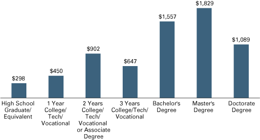
Note: All values shown are significant at the 1 percent level.
Source: Author’s calculations
The link between education and weeks of benefits is not as strong as it was in the wage difference model. The variable coefficients for education levels are mostly significant in the weeks of benefits model. However, the signs are varied and the magnitude is small. The general trend is that higher levels of education will result in less time unemployed. A person with a higher level of education may find work a week or two quicker than someone with low levels of education (see Figure 2).
Figure 2: Influence of Education on Time Spent Unemployed: Effect on Weeks of Unemployment
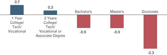
Note: High school and three years of college or technical/vocational school are not significant at the 1 percent level. All values shown are significant at the 1 percent level.
Source: Author’s calculations
The SOC variable results vary. While the coefficients of the SOC variables are significant, the magnitude varies in sign and size in the wage difference model. Some industries, such as engineering and heavy construction, do well in maintaining wages in re-employment (quarterly wage increases of $706 and $600, respectively), while those leaving the military or in the food service industry do poorly (quarterly wage decreases of $2,367 and $1,163, respectively).
The results in the weeks of benefit model are also varied. While most are significant, there is little variation in magnitude. The duration of unemployment is only modestly impacted by the type of industry.
There exists an endogenous link between education and occupation. For example, it is likely that a physician with many years of education will maintain a higher salary than a lower skilled worker. The higher wage compensates the individual for the effort and sacrifice to achieve the level of education required for such a position—in addition to the opportunity cost of lost wages over the years obtaining the education. Simply ignoring this potential source of unobserved heterogeneity can bias estimation results (Baltagi, 1995). An individual’s wage is both a function of the individual and the firm. Since firm-specific data are not available, the inclusion of occupational variables helps control for the influence of this unobserved behavior. Without the occupational code, it would be more difficult to note whether the education is responsible for wage increases or simply correlating with higher wage occupations (such as physicians).
The year variables are controls and attempt to capture influences not expressed by the other variables. Two of the yearly variables are omitted in the study results due to collinearity. The year variables are significant in both models, suggesting temporal influence not captured elsewhere.
Conclusion
The empirical results of historically linked unemployment and wage data confirm the importance of education and its immediate positive impact on wages in the re-employment market. While unemployment has a negative influence on wages, these effects can be somewhat mitigated with higher levels of education. In navigating the re-employment market, not only do higher levels of education present the best opportunity to achieve the best wage outcome when emerging with a new position, but also that a person is likely to find that job quicker. Compared to someone who did not complete a high school education, the value of a bachelor’s degree in the re-employment is a quarterly wage increase of about $1,557. For a high school degree, the quarterly wage increase is $298 for the first position emerging from unemployment. A person will also find the position on average about one week faster with a bachelor’s degree compared to a high school degree.
References
- Acemoglu, D. (2002, March). Technical change, inequality, and the labor market. Journal of Economic Literature, XL, 7-72.
- Baltagi, B. H. (1995). Econometric analysis of panel data. Chichester: Wiley.
- Blackburn, M. L. (1990, Fall). What can explain the increase in earnings inequality among males? Industrial Relations, 29, 441-456.
- Bound, J. and Johnson, G. (1992, June). Changes in the structure of wages in the 1980s: An evaluation of alternative explanations. American Economic Review, 82, 371-392.
- Card, D. (1999). The causal effect of education on earnings. In O. Ashenfelter and D. Card (Eds.), Handbook of labor economics, volume 3 (pp. 1801-1863). Amsterdam: Elsevier.
- Dickens, W. T. and Lang, K. (1985, September). A test of dual labor market theory. American Economic Review, 75, 792-805.
- Dickens, W. T. and Lang, K. (1987). Where have all the good jobs gone? Deindustrialization and the labor market segmentation. In K. Lang and J. Leonard (Eds.), Unemployment and the structure of labor markets. New York. Blackwell.
- Goldin, C. and Margo, R. A. (1992, February). The great compression: The wage structure in the United States at mid-century. Quarterly Journal of Economics, 107, 1-34.
- Karoly, L. A. (1992, February). Changes in the distribution of individual earnings in the United States: 1967-1986. Review of Economics and Statistics, 74, 107-115.
- Katz, L. F. and Murphy, K. M. (1992, February). Changes in relative wages, 1963-1987: Supply and demand factors. Quarterly Journal of Economics, 107, 35-78.
- Kosters, M. (1991). Workers and their wages: Changing patterns in the United States. Washington, DC: American Enterprise Institute.
- Mehta, S. R. (2000, April). Quality of education, productivity changes, and income distribution. Journal of Labor Economics, 18(2), 252-281.
- Revenga, A. L. (1992, February). Exporting jobs? Quarterly Journal of Economics, 107, 255-284.
- Tilak, J. B. G. (1989). Education and its relation to economic growth, poverty, and income distribution: Past evidence and future analysis. Washington, DC: World Bank.
- Teulings, C. N. (1995). The wage distribution model of the assignment of skills to jobs. Journal of Political Economy, 103(2), 280-315.
- Teulings, C. N. (2005). Comparative advantage, relative wages, and the accumulation of human capital. Journal of Political Economy, 113(2), 425-461.
- Thurow, L. (1987, May). A surge in inequality. Scientific American, 256(5), 26-33.
- U.S. Bureau of Economic Analysis. (2015, August). Table data: Real GDP by state (millions of chained 2009 dollars). Retrieved from U.S. BEA website http://www.bea.gov.
- van de Klundert, Th. (1989, October). Wage differentials and employment in a two-sector model with a dual labor market. Metroeconomica, 40, 235-256.